
What is a dipole?
Dipoles appear in many different parts of nature. The simplest to think about is a magnet. By putting iron filing around a bar magnet the so-called field lines (lines of equal potential/magnetism) can be seen.
Bar magnet under paper with iron filing showing the field lines
As a convention we draw lines with arrows from the north to the south pole. The arrows denote the vector (vectors have direction and magnitude i.e. velocity).

Representation of a dipole
Dipoles also appear between charged particles such as a positive nucleus of an atom and the electron, where the arrows go from positive to negative by convention.
Physics of a dipole
A good explanation of how you can work out the field from a dipole can be seen here. Briefly, you can imagine two charged particles a set distance apart. You can work out the fields from simple electrostatics as the sum of the electric field from two points' charges and then as they come close together you end up with a point source dipole. This also works for magnetism, however as Maxwell's equations tell us magnetic flux cannot be created or come from a source so there is no divergence in the field. Mathematically it looks like this:
Thinking about two nuclei close to each other, there will be an addition or subtraction to the overall magnetic field from the magnetic field of the other nuclei. In order to remove this we can look at the z term of the magnetic field (in this case along the axis of the dipole).
We are wanting to see when this contribution goes to zero. Setting this to zero, we see that when the z component of the magnetic field is zero, giving an angle of 54.7 degrees. This is what is called the magic angle.

The plot is a quiver plot with the arrows indicating the field of the magnetic field at that point. You can see where the blue line at 54.7 degrees intersects the arrows that the z component is zero.
In NMR they use rotors that orientate the crystal at the magic angle relative to the magnet field. With the spinning removing any directional effects. This lead to a nice liquid-like NMR peak.
In the Photon Factory we use a pump-probe technique to excite molecules and then see how they decay with time. We polarise the probe light (polarisation is the direction of the electric field) so that it is at the magic angle relative to the pump. This removes any polarisation dependencies from the two incoming beams with the sample (interesting measurements changing the polarisation of the pump and probe. This anisotropy can be used to infer structure of the molecule and other interesting properties).
References
http://bulldog2.redlands.edu/facultyfolder/deweerd/tutorials/Tutorial-QuiverPlot.pdf
Field of a small dipole
http://www.physicsinsights.org/dipole_field_1.html
$ \nabla \cdot B = 0 $
But basically it means that if I were to draw a box around the dipole, the number of field lines going in (flux in) would equal the number of field lines going out (flux out).
Thinking about two nuclei close to each other, there will be an addition or subtraction to the overall magnetic field from the magnetic field of the other nuclei. In order to remove this we can look at the z term of the magnetic field (in this case along the axis of the dipole).
$B_{z}=\frac{|\mu|}{r^{3}}(3cos^{2}\theta -1)$
We are wanting to see when this contribution goes to zero. Setting this to zero, we see that when the z component of the magnetic field is zero, giving an angle of 54.7 degrees. This is what is called the magic angle.
Modelling a dipole
To illustrate this I have a small script I wrote that plots the field lines from a magnet and then integrates a path (in green) where a particle would travel if influenced by the field. The line (in blue) drawn is at 54.7 degrees.
The plot is a quiver plot with the arrows indicating the field of the magnetic field at that point. You can see where the blue line at 54.7 degrees intersects the arrows that the z component is zero.
from pylab import *
from numpy import ma
import numpy as np
import matplotlib.pyplot as plt
import matplotlib
from matplotlib.collections import PatchCollection
import matplotlib.patches as mpatches
from scipy.integrate import odeint

#Size of simulation box
xmax=3.0
xmin=-xmax
NX=19
zmax=3.2
zmin=-zmax
NZ=19


# Setting up the grid
x=linspace(xmin,xmax,NX)
z=linspace(zmin,zmax,NZ)
X, Z = meshgrid(x, z)

#Function that describes the vector field for the integrator
def f(Y,t):
    X, Z = Y
    R = np.sqrt(X**2 + Z**2)
    return((0.5*(3*X*Z/R**5)),(0.5*(3*Z**2/R**5 - 1/R**3)))

#Applying the field to the gridded values
R = np.sqrt(X**2 + Z**2)
Bx = 0.5*(3*X*Z/R**5)
Bz = 0.5*(3*Z**2/R**5 - 1/R**3)

#Had to mask some values so that you don't get large arrows right in the middle
M = zeros((X.shape[0],Z.shape[1]), dtype='bool')
a, b = (NX/2), (NZ/2)
r=3.1

E,W = np.ogrid[-a:NX-a, -b:NZ-b]
print E.shape, W.shape,
mask = E*E + W*W <= r*r
M[mask]=True

#Magic angle line
line = 0.7*x
up = z*0

#Setting up plot
fig = plt.figure()
ax = fig.add_subplot(111)
QP = quiver(X,Z,Bx,Bz,scale=6,headwidth=3,color='grey')

#Integrating paths
for z20 in [-1.0, 1.0]:
    tspan = np.linspace(0, 62, 100)
    z0 = [z20, 0.9]
    zs = odeint(f, z0, tspan)
    plt.plot(zs[:,0],zs[:,1], 'g-') # path

#Box and arrow
arr1 = matplotlib.patches.Arrow(0, -0.5, 0, 1, width=0.4)
rect1 = matplotlib.patches.Rectangle((-0.4,-1),0.8, 2, color='lightblue')
ax.add_patch(rect1)
ax.add_patch(arr1)

#Plotting
plot(x,line,color='blue')
plot(up,z,color='red')
a = title("Magic angle for a dipole")
plt.text(0, 2, "$ B=sin \Theta cos \Theta \hat{x} + (cos^{2} \Theta - 1/3)\hat{z}$",size='large')
savefig('dipole.png',dpi=300)
I also tried out the new streamlines plot in matplotlib. |
| Field lines of a magnet (red) with line drawn at the magic angle (blue) seen intersecting the field lines exactly where the z component (upwards component) of the field is zero. |
#Setting up new range for streamlines
xmax=3.0
xmin=-xmax
NX=100
zmax=3.2
zmin=-zmax
NZ=100

x=linspace(xmin,xmax,NX)
z=linspace(zmin,zmax,NZ)
X, Z = meshgrid(x, z)

#Function for the vector field
R = np.sqrt(X**2 + Z**2)
Bx = 0.5*(3*X*Z/R**5)
Bz = 0.5*(3*Z**2/R**5 - 1/R**3)

#Unset mask for streamplot
M[mask]=False

fig = plt.figure()
ax = fig.add_subplot(111)

#New streamplot in matplotlib
QS = streamplot(X,Z,Bx,Bz,density=[1.3,1.3],linewidth=1,color='red',minlength=0.3)

arr1 = matplotlib.patches.Arrow(0, -0.5, 0, 1, width=0.4)
rect1 = matplotlib.patches.Rectangle((-0.4,-1),0.8, 2, color='lightblue')
ax.add_patch(rect1)
ax.add_patch(arr1)

plot(x,line,color='blue',)
plot(up,z,color='green',linewidth=1.5)
a = title("Magic angle for a dipole potential")
plt.text(0.2, 2.8, "$ B=sin \Theta cos \Theta \hat{x} + (cos^{2} \Theta - 1/3)\hat{z}$",size='large')

savefig('dipole_streamlines.png',dpi=300)
We we see is that at the magic angle we remove all of the effects of the magnetic field in the z direction on the particle.In NMR they use rotors that orientate the crystal at the magic angle relative to the magnet field. With the spinning removing any directional effects. This lead to a nice liquid-like NMR peak.
 |
| http://en.wikipedia.org/wiki/Magic_angle_spinning |
In the Photon Factory we use a pump-probe technique to excite molecules and then see how they decay with time. We polarise the probe light (polarisation is the direction of the electric field) so that it is at the magic angle relative to the pump. This removes any polarisation dependencies from the two incoming beams with the sample (interesting measurements changing the polarisation of the pump and probe. This anisotropy can be used to infer structure of the molecule and other interesting properties).
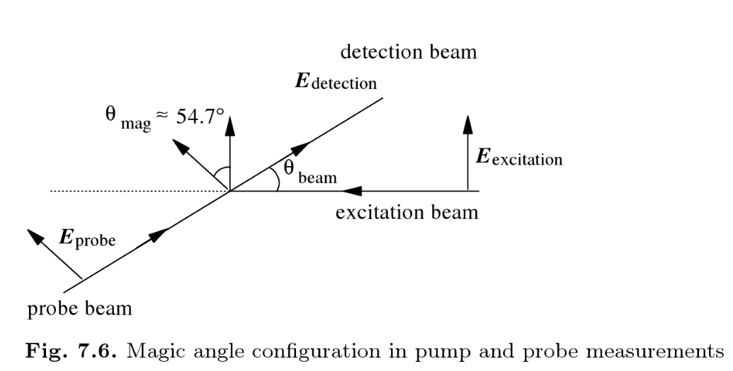 |
| Menzel R., "Photonics: Linear and Nonlinear Interactions of Laser Light and Matter" |
http://bulldog2.redlands.edu/facultyfolder/deweerd/tutorials/Tutorial-QuiverPlot.pdf
Field of a small dipole
http://www.physicsinsights.org/dipole_field_1.html


