Sunday, 12 November 2017

Nanotechnology right under our noses

Image sources: link, linklink
Nanotechnology conjures up images of tiny machines able to deliver drugs to the body, produce clean energy or take over the world - depending on who you talk to. The reality is that many of the nanostructures that scientists currently use in the lab have already been used for millennia.

In the past, gold nanoparticles were used to produce brilliant reds in stained glass windows and nanoscale tubes were woven into Damascus steel to make strong, sharp swords. These technologies were used without full knowledge of the processes involved, or safety concerns; however, the recent breakthrough in nanotechnology is our understanding and control of nanoscale structures.

My colleagues and I at the Department of Chemical Engineering and Biotechnology have found a common nanostructure that unites a variety of carbon materials, many of which are right under your nose. Water and air filters use activated carbon and vehicles produce soot - even your tennis racket and bike that contain carbon fibres.

You might be familiar with the layered structure of graphite: carbon atoms are arranged hexagonally in sheets that can easily glide past each other. This makes graphite a great material for pencil lead or a solid lubricant, but not as a filter or a bike frame. When graphite starts to become curved and interlinked is when the structure takes on its exceptional and diverse properties.

We ran quantum chemical calculations on the university’s supercomputers to understand what occurs when curvature is integrated into graphitic sheets through the replacement of a hexagonal ring of carbon with a pentagonal ring. This leads to a permanent bend in the structure that shuttles electrons from one side of the sheet to the other. This electric polarisation significantly increases the interaction of curvature-containing carbon material with molecules and itself, explaining how a relatively inert graphite can become strong and porous.

The next step for us is to explore how we can use our discoveries to reduce the emission of soot from vehicles, improve water filtration and improve the many carbon nanostructures that are right under our noses.

Thursday, 9 November 2017

Polar aromatic molecules


We have recently published a paper on an interesting class of curved aromatic molecules. Here is an interactive 3D model of one of the molecules we studied. Click and drag to rotate the model in 3D, zoom in and out with the mousewheel.


In short
  • We found that this curving of the molecules shifted the electrons from the concave to the convex side of the molecule which makes quite a large electric field. 
  • This is quite a strange finding mainly because most aromatic molecules are usually considered electrically non-polar.
  • These curved molecules have been spotted (using electron microscopes) in soot particles, carbon battery electrodes and carbon water filters. 
  • The electric field around these molecules will have a huge impact on how they interact with polar molecules such as water and many pollutants the electric field will also provide significant interactions with ions such as lithium used in batteries. 
You can read the full preprint of the paper for free on our website

Want to know more about polar molecules, why these aromatic molecules are polar and more about what this could mean for carbon research please read on.

What are polar molecules?


You may have heard that water is polar and other substances are non-polar like oil. Polar refers to the electric field around the molecule which has two poles a negative and a positive pole/end. For two opposite charges the potential is plotted below where red denotes a negative potential and blue a positive potential. The lines are lines of constant potential and are like contour lines on a map of a volcano denoting regions with the same value/height.

Credit: link
The dipole moment is defined as the distance the charges are separated multiplied by the difference between the two charges. Two opposite elementary charges (charge of an electron) separated by 0.1 nm gives a dipole moment of 4.8 D (debyes).

The atomic nuclei are small and positively charged and can be considered as point charges however the electrons are not well defined but spread out over space due to quantum mechanics. In this case we can define the molecular dipole as a sum of the dipole moment from the nuclei, as point charges, and the dipole from the electron density which can be unevenly shared between the atoms. The picture below on the left shows the electron density in gray at a certain value (kind of like a 3D contour) as a surface for hydrochloric acid. You can see more electron density on the chlorine atom, this is mainly because the chlorine nucleus has a charge of +17 compared with the hydroge nuclei which only has a charge +1, but there is also even more electron density on the chlorine nuclei than enough to cancel the positive nuclei making the potential on this surface more negtaive on the chlorine side than the hdyrogen side (seen in the figure below right). Giving HCl a dipole moment of 1.08 D. 


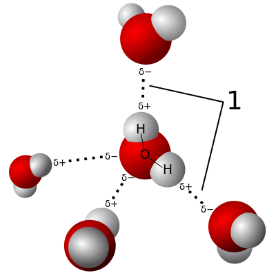
The cloud of electrons becomes very repulsive when molecules approach each other past the surface we have drawn. So you can think of this surface as the place where the molecules will touch each other (this surface is near the electron density value of 0.001 eÅ$^{-3}$). You might know that opposite charges attract so if you line up two molecules of HCl with the negative chlorine of one pointing towards the positive hydrogen of the other they will be attract each other. Below is a picture showing the attractive and repulsive ways of orienting two polar molecules. The Greek delta character δ is used to denote partially charged regions as the ends of the molecule do not have point charge of +1 but are only partially charged.
Credit: link and recoloured
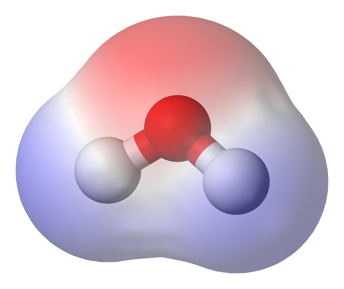
Water is the most commonly known polar molecule. Below I am plotting the electric field around a water molecule along with the potential at the interaction surface. 


As these is a assymmetry to the electric potential (i.e. one side is positive and the other negative) water has a dipole moment of 1.85 D in the gas phase. This allows water to strongly interact with other water molecules and is what holds water together as a liquid at room temperature when similar sized molecules such as methane are no where near being liquid. Methane is a gas at room temperature and needs to be cooled to -161.5 °C before it becomes a liquid. Below is an animation of water molecules attracting each other (often called a hydrogen bond). Apart from the amazing fact of being a liquid at room temperature water forms a strange cage structure when it freezes which takes up more room than the liquid meaning it is less dense and allows solid water to uniquely float on the liquid.

Credit: CSIC


Credit: Qwerter

If you have a balloon handy you can do a simple experiment to convince yourself that water is polar. Rubbing a balloon with a cloth or on your head removes positive charge and leaves the balloon with a negative charge. Holding the balloon near a stream of water the positive side of the water molecule will be attracted to the negative charge on the balloon and it will bend the water toward itself.

Credit: Link
To put a scale in your mind as to the common range of dipole moments I have added the table below.


Table of the dipole moment in Debye units (1 D = 3.336×10^-30 C m) taken from Israelachvili 1992
Molecule Formula Dipole moment
Ethane $\text{C}_2\text{H}_6$ 0
Benzene $\text{C}_6\text{H}_6$ 0
Carbon tetrachloride $\text{CCl}_4$ 0
Carbon dioxide $\text{CO}_2$ 0
Chloroform $\text{CCl}_3$ 1.06
Hydrochloric acid $\text{HCl}$ 1.08
Ammonia $\text{NH}_3$ 1.47
Phenol $\text{C}_6\text{H}_5\text{OH}$ 1.5
Ethanol $\text{C}_2\text{H}_5\text{OH}$ 1.7
Water $\text{H}_2\text{O}$ 1.85
Cesium Chloride $\text{CsCl}$ 10.4

You will notice the aromatic molecule benzene does not have a dipole moment in the next section we will explore why this is the case.

Are planar aromatic molecules polar?


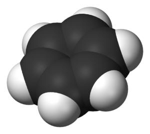
Benzene is the simplest aromatic molecule. It is made of six carbon atoms arranged into a hexagonal ring (below left). Adding six more hexagonal rings of carbon you can produce coronene a large polycyclic aromatic hydrocarbon with seven hexagonal rings of carbon (below right).


Plotting below the electrostatic potential of these two molecules looking side on (perpendicular to the aromatic plane) the electric field around planar aromatic molecules can be viewed. Around the hydrogen atoms, often called the rim of the PAH, the potential is positive. The top and bottom near the carbon atoms is negative. This can be explained by the bonding but we will leave this for another post.


As you can see there is no one side that is negative and another that is positive (no assymmetry). The potentials are mirror images. There is no net dipole moment for planar aromatic molecules i.e. they are non-polar. This means they will only have weak interactions with polar molecules such as water making aromatics insoluble in water.

This arrangement of charged regions is called a quadrupole and is one moment higher than the dipole. Below are some point charge representations of a quadrupole and a contour plot of a quadrupole.


So how can we make an aromatic molecule polar. The next section will show that curvature integration is the key.

Curved aromatics are polar


Curvature is integrated into aromatic molecules when a non-hexagonal ring of carbon atoms is integrated into the normally closed 

Corannulene is experimentally known to contain a dipole moment of 2.07 D. This is quite a large dipole moment close to that of water. Below I have plotted the electric field around water, corannulene and coronene far away from the molecules (around 4 nm).

Comparing corannulene to water a similar potential is seen at the far field, however, close to the molecule there is a negative potential near the concave side of the bowl. Comparing corannulene to coronene the positive region around the hydrogen atoms is similar in both molecules, however, there is a shift of the negative potential to the convex surface of the curved corannulene. This turns out to be due to an effect called flexoelectricity. By flexing the molecule you shift electrons from the concave to the convex surface leading to the dipole you see.

We used a supercomputer to calculate the electron density around some very large curved aromatic molecules. From this we could determine the dipole moment with very good accuracy (less than 2% error for corannulene compared with experiment). The figure below shows the strong scaling of the dipole moment with the size of the molecules. The size range found in soot and other carbon materials is around 10-20 aromatic rings shown as the shaded grey area. This indicates that curved fragments in carbon materials can have a significant dipole moment of 2-6 D.


Why is this result so exciting?


There are many carbon materials that contain these curved aromatic molecules such as soot (pollutant from engines that contributes to global warming), carbon blacks (used in inks and tires), activated carbon (used in water filters, they are also used as an antidote to poisons as they are very good at sucking up organic molecules and metals) and battery carbon electrodes. To date very few people have considered these molecules to contain a dipole moment and what impact that has on their performance.
The considerable dipole moment we predict will have a huge impact on how the carbon materials interact with other molecules here are a few potential important interactions.
  • In batteries positively charged lithium ions will interact strongly with the dipole moment on the curved molecules.
  • In soot formation charged chemi-ions will interact strongly with curved aromatic molecules in the flame.
  • In activated carbon a strong interaction is expected between the dipole moment and adsorbents that are charged or polar.  
If you are interested in how you can include these effects into computer simulations of carbon systems read on.

Simulating carbon materials with curvature in the computer


Many important properties of carbon materials could be potentially optimised if we can tune the curvature in carbon materials. A simple mathematical representation in the computer is needed to model these properties. A common representation of the electric field in computer simulations around the molecule is to use point charges at each atom (usually much less than an atomic charge) and then fit the electrostatic potential around the molecule by adjusting these charges to match the electric field far away from the molecule. We usually also add a repulsive mathematical function so that the molecule cannot get too close to another. This means the potential is only important outside this region which can be thought of as an interaction surface. This means we need to correctly describe the electrostatic at and outside the interaction surface. A previous PhD student Tim Totton along with Dr. Alston Misquitta developed a forcefield for planar PAH molecules and found that atomic centred point charges do a good job of describing the electric field around these molecules. Below is a picture of the electric potential around coronene calculated from a full quantum mechanical simulation (DFT) and using point charges centred at each atom. The far right shows an overlay of the two showing remarkable agreement.


When we tried the same fitting of the electrostatic potential for corannulene using atom centred point charges we found a very bad fit. The first problem was the magnitude of the dipole moment was reduced to 1.73 D. The reason the fit was so poor is due to the flexoelectric effect which occurs perpendicular to the rings. This means dipoles must be included on the pentagonal carbon atoms to correctly describe these. We made use of atom-centred multipoles (monopole+dipole+quadrupole) to correctly describe the polarisation and the quadrupoles provide better description of the potential around the hydrogen atoms. Below is a figure of the potential around corannulene for point charges and for multipoles.


These atom centred multipoles descriptions of molecular electrostatics have recently been integrated into different molecular dynamics packages such as Tinker, OpenMM and DL_POLY. Get in contact if you are interested in simulating a certain carbon system and I would be happy to work with you on it.

Wednesday, 1 November 2017

Curving aromatic molecules

Credit: link
Aromatic molecules such as benzene and coronene (shown above) contain a hexagonal arrangement of carbon atoms. This gives a flat planar structure due to the geometry of hexagonal rings which are able to tessellate in two dimensions (see the tessellating tiles in the picture below). You can think of these hexagonal aromatics being like a flat saucers.


Credit: Paula Soler-Moya
A hexagonal arrangement of carbon atoms is the most stable (making grapite the most stable form of carbon, being made up of hexagonal sheets of carbon). The molecule shown below left (benzo(ghi)fluoranthene) would at lower temperatures and over longer times rearrange and form a completely hexagonal structure but in the formation of soot in a flame a faster reaction has been found with acetylene which forms the less stable corannulene molecule with a pentagon trapped within. Integration of this non-hexagonal rings into a hexagonal lattice does not leads to a net that can be nicely tessellated on a 2D surface but leads to a 3D warped structure - a bowl-like geometry. I have embeded an interactive 3D models of these two molecules so you can see this 3D curvature for yourself (click and drag to move the grey models around and zoom with your mouse wheel).


Related image
Credit: Ikea

The curvature leads to many interesting physical properties of these molecules such as a permanent dipole moment and interesting electrical properties which might make these molecules useful for organic light emitting diodes or as electrical connections between molecular computers and metal contacts. More to come...

Molecular dynamics in Python

Molecular dynamics

Molecular simulations have been heralded as the new computational microscope that are helping us understand how molecules interact with each other and how they self assemble into complex structures. A molecular dynamics simulation is a particular type of simulation which generally approximates the intermolecular forces/energy using mathematical functions. The impact of temperature is often included (which usually drives molecules apart) and the interplay between this thermal energy and the intermolecular energy gives rise to the self assembly processes.

There are many different applications to molecular dynamics including describing the interactions between drugs and protein binding sites and describing the self-assembly of molecular systems like lipid bilayers and colloids. Colleagues and I have used molecular dynamics to simulate the self assembly of soot and the dynamics of polymers for CO2 separation. I have put this short example together using the simplest potential - the Lennard-Jones potential. This potential describes the attraction at long distances and repulsion at short distances and can model the behaviour of gases such as argon and helium quite well. This example is based on the fortran code written by Furio Ercolessi, SISSA, Trieste. This example is written in the ipython notebook and the python scripts can be copied and run on any computer with python 2 installed along with the numpy and matplotlib libraries.

Molecular dynamics basics

Most molecular dynamics programs use classical approximations (Newtonian mechanics) to describe the energy of the system as a function of the positions of the atoms/particles.

$$ E(\textbf{r}) $$

We can use Newton's second law to describe the motion of the particles through time.

$$ F = m \textbf{a} = m \frac{d^{2}\textbf{v}}{dt^{2}}$$

The force can be calculated in one dimension by taking the derivative with respect to $x$ (or in three dimensional vector notation, the gradient $\nabla$) of the energy.

$$ F = -\frac{dE}{dx} = -\nabla E(\textbf{r}) $$

So the first step is to calculate the forces on the particles by describing the intermolecular potential energy.

Lennard-Jones potential

The potential energy of the 12-6 Lennard-Jones potential is given as

$$ E_{LJ}(r)=4\epsilon\left[ \left( \frac{\sigma}{r}\right)^{12}- \left( \frac{\sigma}{r}\right)^{6} \right] $$

$ \sigma $ is the radius where the potential is zero and is defined as the van der waals radius. $ \epsilon $ is the energy minimum of the interaction (see the figure below).

We don't want to compute long range interactions as they will be negligible. We therefore apply a cutoff past $r/\sigma=2.5$. However, as the particles move past the cutoff distance there will be a small jump in the energy, which is not realistic, so we shift the potential so that the potential goes to zero at $r/\sigma=2.5$.

Below is a plot of the Lennard-Jones potential with the shifted potential shown for comparison.

In [163]:
#Import a plotting libraries and a maths library 
import matplotlib.pyplot as plt
import numpy as np
%matplotlib inline

r = np.linspace(0.01,3.0,num=500) # Make a radius vector
epsilon = 1 # Energy minimum
sigma = 1 # Distance to zero crossing point
E_LJ = 4*epsilon*((sigma/r)**12-(sigma/r)**6) # Lennard-Jones potential

plt.figure(figsize=[6,6])
plt.plot(r,E_LJ,'r-',linewidth=1,label=r" $LJ\; pot$") # Red line is unshifted LJ

# The cutoff and shifting value
Rcutoff = 2.5
phicutoff = 4.0/(Rcutoff**12)-4.0/(Rcutoff**6) # Shifts the potential so at the cutoff the potential goes to zero

E_LJ_shift = E_LJ - phicutoff # Subtract the value of the potential at r=2.5

plt.plot(r[:415],E_LJ_shift[:415],'b-',linewidth=1,label=r"$LJ\; pot\; shifted$") # Blue line is shifted

#Plot formatting
plt.rc('text', usetex=True)
plt.rc('xtick', labelsize=20) 
plt.rc('ytick', labelsize=20) 
plt.title(r"$Lennard-Jones\; potential$",fontsize=20)
plt.xlim([0.0,3.0])
plt.ylim([-1.5,1.5])
plt.ylabel(r"$E_{LJ}/\epsilon$",fontsize=20)
plt.xlabel(r"$r/\sigma$",fontsize=20)
plt.legend(frameon=False,fontsize=20)
plt.axhline(0, color='grey',linestyle='--',linewidth=2)
plt.axvline(1, color='grey',linestyle='--',linewidth=2)
Out[163]:
<matplotlib.lines.Line2D at 0x10b68fac8>

Reduced units

By choosing our units we can remove any constants and get a general behaviour for all gases. Mass, sigma, epsilon and the Boltzmann constant are set to equal one. Reduced coordinates are used for the other variables which are derived from the parameters set to one.

$$ x^{*} = \frac{x}{\sigma} $$$$ v^{*} = v\frac{t^{*}}{\sigma} $$$$ t^{*} = t\left(\frac{\epsilon}{m \sigma^{2}} \right)^{1/2} $$$$ E^{*} = \frac{E}{\epsilon} $$$$ F^{*} = f\frac{\sigma}{\epsilon} $$$$ P^{*} = P \frac{\sigma^{3}}{\epsilon}$$$$ \rho^{*} = \rho \sigma^{dimensions} $$$$ T^{*} = T \frac{k_{b}}{\epsilon} $$

Where $k_{b}$ is Boltzmann's constant.

This may seem complicated but it allows all of the equations to be written very simply in the program. This also gives us physical insight - for example, the reduced temperature is the ratio of the thermal energy $k_{B} T$ to the energy of the intermolecular interactions $\epsilon$.

Periodic boundary conditions

Periodic boundary conditions allow for an approximation of an infinitely sized system by simulating a simple unit cell. This is illustrated below. The black box is the only cell we simulate; the tiled images around it are there for illustration. The green particle moves past the top boundary of the unit cell and are moved to the bottom of the box with the same velocity (illustrated by the red dashed line). This boundary condition keeps the volume and number of particles constant in the simulation.

Limiteperiodicite.svg
By I, Grimlock, CC BY-SA 3.0, Link

Calculating the forces

As mentioned above, the forces between particles can be calculated from the derivative/gradient of their potential energy. $\textbf{F}=-\frac{1}{r}\nabla E(\textbf{r})$ (in spherical coordinates)

$$ \textbf{F} = -\frac{1}{r}\nabla E_{LJ}(\textbf{r}) = -\frac{1}{r}\frac{d E_{LJ}}{d \textbf{r}} = -24\left[2\left(\frac{\sigma}{\textbf{r}}\right)^{14} - \left(\frac{\sigma}{\textbf{r}}\right)^{8}\right] $$

Periodic boundary conditions have to be considered when we compute the forces between particles because a particle near the boundary of the unit cell has to be able to feel the force from a particle on the other side of the unit cell. For example, the pink particle above will feel the force from the green particle, even though they are far from each other because they are near opposite boundaries.

In order to easily implement periodic boundary conditions, scaled box units are used so that the particle positions are always between -0.5 and 0.5. If the distance between the particles is greater than half the scaled box units, the interaction with the particle in the next box are considered.

In [122]:
def Compute_Forces(pos,acc,ene_pot,epsilon,BoxSize,DIM,N):
    # Compute forces on positions using the Lennard-Jones potential
    # Uses double nested loop which is slow O(N^2) time unsuitable for large systems
    Sij = np.zeros(DIM) # Box scaled units
    Rij = np.zeros(DIM) # Real space units
    
    #Set all variables to zero
    ene_pot = ene_pot*0.0
    acc = acc*0.0
    virial=0.0
    
    # Loop over all pairs of particles
    for i in range(N-1):
        for j in range(i+1,N): #i+1 to N ensures we do not double count
            Sij = pos[i,:]-pos[j,:] # Distance in box scaled units
            for l in range(DIM): # Periodic interactions
                if (np.abs(Sij[l])>0.5):
                    Sij[l] = Sij[l] - np.copysign(1.0,Sij[l]) # If distance is greater than 0.5  (scaled units) then subtract 0.5 to find periodic interaction distance.
            
            Rij = BoxSize*Sij # Scale the box to the real units in this case reduced LJ units
            Rsqij = np.dot(Rij,Rij) # Calculate the square of the distance
            
            if(Rsqij < Rcutoff**2):
                # Calculate LJ potential inside cutoff
                # We calculate parts of the LJ potential at a time to improve the efficieny of the computation (most important for compiled code)
                rm2 = 1.0/Rsqij # 1/r^2
                rm6 = rm2**3.0 # 1/r^6
                rm12 = rm6**2.0 # 1/r^12
                phi = epsilon*(4.0*(rm12-rm6)-phicutoff) # 4[1/r^12 - 1/r^6] - phi(Rc) - we are using the shifted LJ potential
                # The following is dphi = -(1/r)(dV/dr)
                dphi = epsilon*24.0*rm2*(2.0*rm12-rm6) # 24[2/r^14 - 1/r^8]
                ene_pot[i] = ene_pot[i]+0.5*phi # Accumulate energy
                ene_pot[j] = ene_pot[j]+0.5*phi # Accumulate energy
                virial = virial + dphi*np.sqrt(Rsqij) # Virial is needed to calculate the pressure
                acc[i,:] = acc[i,:]+dphi*Sij # Accumulate forces
                acc[j,:] = acc[j,:]-dphi*Sij # (Fji=-Fij)
    return acc, np.sum(ene_pot)/N, -virial/DIM # return the acceleration vector, potential energy and virial coefficient
            

Temperature

Temperature is a macroscopic quantity. Microscopically it is less well defineddue to the low number of particles. However, if we use the kinetic energy of the parameters we can calculate the temperature.

$$ E_{K}=\frac{1}{2} mv^{2} $$$$ k_{B} T = \frac{2}{3}\sum_{N}E_{K} $$

Where we sum over all $N $ atoms. We will use this in order to scale the velocities to maintain a constant temperature (remember we are using reduced units so $k_{B}=1$ and $m=1$).

The function below calculates the temperature given the velocity of the atoms/particles.

In [123]:
def Calculate_Temperature(vel,BoxSize,DIM,N):
    
    ene_kin = 0.0
    
    for i in range(N):
        real_vel = BoxSize*vel[i,:]
        ene_kin = ene_kin + 0.5*np.dot(real_vel,real_vel)
    
    ene_kin_aver = 1.0*ene_kin/N
    temperature = 2.0*ene_kin_aver/DIM
    
    return ene_kin_aver,temperature

Molecular dynamics program

The molecular dynamics program contains the instructions for the computer to use to move the particles/atoms through time. Most often this is written in Fortran and C; these compiled languages are orders of magnitude faster than Python, however a scripting language like Python is helpful to provide understanding about how molecular dynamics is implemented.

The main steps in a molecular dynamics simulation are:

  1. Initialise the position of particles
  2. Calculate the pairwise forces on the particles by calculating the gradient of the potential energy $ F = \nabla E(\textbf{r})=1/r\partial E(\textbf{r})/\partial r$
  3. Compute the new positions by integrating the equation of motion (we will use the velocity Verlet algorithm)
  4. Apply a thermostat to maintain the temperature at the set value (we will use the velocity scaling for temperature control)
  5. Go back to step 2, recompute the forces and continue until the maximum number of steps

Initialising the particles

In [161]:
DIM = 2 # Dimensions
N = 32

BoxSize = 10.0#6.35 

volume  = BoxSize**DIM
density = N / volume
print("volume = ", volume, " density = ", density)

pos = np.zeros([N,DIM])
        
pos = np.genfromtxt('output.dat',skip_header=1) # Load positions from file
pos = pos[:,:DIM]/BoxSize

MassCentre = np.sum(pos,axis=0)/N

for i in range(DIM):
    pos[:,i] = pos[:,i]-MassCentre[i]
    
    
volume =  100.0  density =  0.32

Integrating the equations of motion

We will make use of the velocity Verlet integrator which integrates Newton's equations of motion in 1D:

$$ \frac{dx}{dt}=v\; and \; \frac{dv}{dt}=\frac{dF(x)}{m} $$

The velocity Verlet algorithm spilts the velocity update into two steps intially doing a half step then modifing the acceleration and then doing the second velocity update. Written in full, this gives:

  1. Calculate $x(t+\Delta t) = x(t)+v\left(t+\frac{1}{2}\right)\Delta t$
  2. Calculate $v\left(t+\frac{1}{2}\Delta t\right)= v(t)+\frac{1}{2}a(t)\Delta t $
  3. Derive $a(t+\Delta t)$ from the interaction potential using $x(t+\Delta t)$
  4. Calculate $v(t+\Delta t)=v\left(t+\frac{1}{2}\right)+\frac{1}{2}a(t+\Delta t) \Delta t$

Between step 1 and 2 we rescale the velocities to maintain the temperature at the requested value.

The output is saved in the same folder as the ipython notebook as traj.xyz and can be opened by Avogadro or VMD.

In [155]:
# Setting up the simulation
NSteps=10000 # Number of steps
deltat = 0.0032 # Time step in reduced time units
TRequested = 0.5# #Reduced temperature
DumpFreq = 100 # Save the position to file every DumpFreq steps
epsilon = 1.0 # LJ parameter for the energy between particles

# Main MD loop
def main(pos,NSteps,deltat,TRequested,DumpFreq,epsilon,BoxSize,DIM):
    
    # Vectors to store parameter values at each step
    N = np.size(pos[:,1])
    ene_kin_aver = np.ones(NSteps)
    ene_pot_aver = np.ones(NSteps)
    temperature = np.ones(NSteps)
    virial = np.ones(NSteps)
    pressure = np.ones(NSteps)
    ene_pot = np.ones(N)

    vel = (np.random.randn(N,DIM)-0.5)
    acc = (np.random.randn(N,DIM)-0.5)

    # Open file which we will save the outputs to
    f = open('traj.xyz', 'w')
    
    for k in range(NSteps):
        
        # Refold positions according to periodic boundary conditions
        for i in range(DIM):
            period = np.where(pos[:,i] > 0.5)
            pos[period,i]=pos[period,i]-1.0
            period = np.where(pos[:,i] < -0.5)
            pos[period,i]=pos[period,i]+1.0

        # r(t+dt) modify positions according to velocity and acceleration
        pos = pos + deltat*vel + 0.5*(deltat**2.0)*acc # Step 1

        # Calculate temperature
        ene_kin_aver[k],temperature[k] = Calculate_Temperature(vel,BoxSize,DIM,N)

        # Rescale velocities and take half step
        chi = np.sqrt(TRequested/temperature[k])
        vel = chi*vel + 0.5*deltat*acc # v(t+dt/2) Step 2

        # Compute forces a(t+dt),ene_pot,virial
        acc, ene_pot_aver[k], virial[k] = Compute_Forces(pos,acc,ene_pot,epsilon,BoxSize,DIM,N) # Step 3

        # Complete the velocity step 
        vel = vel + 0.5*deltat*acc # v(t+dt/2) Step 4

        # Calculate temperature
        ene_kin_aver[k],temperature[k] = Calculate_Temperature(vel,BoxSize,DIM,N)

        # Calculate pressure
        pressure[k]= density*temperature[k] + virial[k]/volume
        
        
        # Print output to file every DumpFreq number of steps
        if(k%DumpFreq==0): # The % symbol is the modulus so if the Step is a whole multiple of DumpFreq then print the values

            f.write("%s\n" %(N)) # Write the number of particles to file
            # Write all of the quantities at this step to the file
            f.write("Energy %s, Temperature %.5f\n" %(ene_kin_aver[k]+ene_pot_aver[k],temperature[k]))
            for n in range(N): # Write the positions to file
                f.write("X"+" ")
                for l in range(DIM):
                    f.write(str(pos[n][l]*BoxSize)+" ")
                f.write("\n")
            
            if(DIM==2):
                import matplotlib.pyplot as plt
                from IPython import display
                plt.cla()
                plt.xlim(-0.5*BoxSize,0.5*BoxSize)
                plt.ylim(-0.5*BoxSize,0.5*BoxSize)
                for i in range(N):
                    plt.plot(pos[i,0]*BoxSize,pos[i,1]*BoxSize,'o',markersize=20,)
                display.clear_output(wait=True)
                display.display(plt.gcf())
        #print(ene_kin_aver[k], ene_pot_aver[k], temperature[k], pressure[k]) 

    f.close() # Close the file
    
    return ene_kin_aver, ene_pot_aver, temperature, pressure, pos
In [157]:
ene_kin_aver, ene_pot_aver, temperature, pressure, pos = main(pos,NSteps,deltat,TRequested,DumpFreq,epsilon,BoxSize,DIM)
Done
In [158]:
# Plot all of the quantities
def plot():
    plt.figure(figsize=[7,12])
    plt.rc('xtick', labelsize=15) 
    plt.rc('ytick', labelsize=15)
    plt.subplot(4, 1, 1)
    plt.plot(ene_kin_aver,'k-')
    plt.ylabel(r"$E_{K}$", fontsize=20)
    plt.subplot(4, 1, 2)
    plt.plot(ene_pot_aver,'k-')
    plt.ylabel(r"$E_{P}$", fontsize=20)
    plt.subplot(4, 1, 3)
    plt.plot(temperature,'k-')
    plt.ylabel(r"$T$", fontsize=20)
    plt.subplot(4, 1, 4)
    plt.plot(pressure,'k-')
    plt.ylabel(r"$P$", fontsize=20)
    plt.show()

plot()
In [159]:
print("Temperature = ", np.average(temperature), "+-", 2*np.std(temperature))
Temperature =  0.499976604421 +- 0.00580962776371
In [160]:
print("Pressure = ", np.average(pressure), "+-", 2*np.std(pressure))
Pressure =  0.273148208667 +- 0.365424653066

The thermostat appears to be holding the temperature close to the requested value of $T^{*}=0.5$.

In [166]:
# Stylings from http://lorenabarba.com
from IPython.core.display import HTML
def css_styling():
    styles = open("custom.css", "r").read()
    return HTML(styles)
css_styling()
Out[166]:

Implementation in LAMMPS

Lammps is a very fast molecular dynamics package. The input file is below and performs a much longer simulation in less than a minute. At the top of the this article is the animated video from the simulation where the temperature was reduced from $T^*=$1.0 to $T^*=$0.2 showning the nucleation of a crystal.

# 2d Lennard-Jones melt

variable    x index 1
variable    y index 1
variable    z index 1

variable    xx equal 40*$x
variable    yy equal 20*$y
variable    zz equal 20*$z

units        lj
atom_style    atomic
dimension 2

lattice        hex 0.8442 #Set the lattice vector
region        box block 0 ${xx} 0 ${yy} 0 1 # Make region for the periodic box
region        two block 5 15 5 15 0 1 # Make a region for where the atoms will begin
create_box    1 box
create_atoms    1 region two # Create the atoms
mass        1 1.0

velocity    all create 1.44 87285 loop geom # Set their initial velocity which will be scaled during the simulation

pair_style    lj/cut 2.5 # Define the intermolecular interaction with the Lennard-Jones function with a cutoff of 2.5
pair_coeff    1 1 1.0 1.0 2.5 # Setting the sigma and epsilon values

# This neighbor list improves the efficiency of the calculation by only calculating interactions with particles within cutoff+0.3
neighbor    0.3 bin 
neigh_modify    delay 0 every 20 check no

dump    1    all xyz 200 dump.lj #Saves the trajectory to a file to open in VMD

fix        1 all nve # Performs an integration to move the sample through time
fix        2 all enforce2d # Make sure there is no forces in the z direction 
fix        3 all temp/rescale 1 1.0 0.2 0.02 0.5 # This rescales the velocity to keep the temperature constant.
run        1000000 #run for this number of steps the default timestep for lj is 0.005 tau